Formula - Return month as text from a date cell.

AGillespie · 06/13/18

I want to use the formula:

=TEXT(*CELL WITH DATE*,"mmmm")

But this doesn't seem to be a valid formula on Smartsheet.

So if I have a cell with the date "01/01/19" - I want it to show "January" in another cell.

John C Murray · 08/22/23

If you only need three digit month names the formula is much simpler:

=MID("JanFebMarAprMayJunJulAugSepOctNovDec", (Mth@row * 3) - 2, 3)

J. Craig Williams · 06/13/18

Here's what I do:

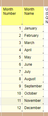
I have a sheet called "Date Tables". In that sheet I have a column for Month Number and another for Month Name.

1 January

2 February

3 March

4 April

5 May

6月6日

7 July

8 August

9 September

10 October

11 November

12 December

I use X-Sheet references to get the name from the number.

Like this:

=IFERROR(INDEX({Date Tables | Month Name}, MATCH(MONTH(Start@row), {Date Tables | Month Num}, 0)), "")

You only need to set up the X-Sheet references once per sheet.

Alternatively, you can build a complicated nested-if statement, but I won't.

Craig

AGillespie · 06/13/18

Hey,

非常感谢,但是,哇,一只老鼠her convoluted work-around for what you'd think should be a simple formula. I'll try it out.

J. Craig Williams · 06/13/18

There are posts on the Community with the nested-if example. That's worse.

Before X-Sheet references, I would have the data on a hidden area of the sheets.

Since I just copy/paste the formulas, it only take a minute or two to setup a new sheet for the functionality.

Craig

bkhunt22 · 07/03/18

Hey Craig - I have created my date tables sheet, and am trying to build out my formula to replicate this but am having a hard time dissecting your formula to adjust to my sheet names, etc.

Can you break it down for me?

=IFERROR(INDEX({Date Tables | Month Name}, MATCH(MONTH(Start@row), {Date Tables | Month Num}, 0)), "")

Thank you!

J. Craig Williams · 07/03/18

Yep.

=IFERROR(INDEX({Date Tables | Month Name}, MATCH(MONTH(Start@row), {Date Tables | Month Num}, 0)), "")

MATCH( the month of the date in the [Start] column on this row with the column of data called {Date Tables | Month Num} -- which is a single column of the numbers 1-12.

The last argument (0) is habit and is looking at an unsorted list.

This returns the row number (within the table), so 2018-06-06 would search for 6 and find it on the 7th row (since my table has a header)

INDEX takes that row number (in our example 7) and returns the matching value from the column of data called {Data Tables | Month Name} -- another single column with the text of the month's names.

I use INDEX(...,MATCH()) in case someone decides to change the order of the columns, put something between them, or otherwise mess up what I might think of as a beautiful table, perfect in form.

Lastly, I wrap it in IFERROR (returning a blank if one is found) because MONTH() throws an error on blanks.

See image for what the data looks like

Craig

Barry Bowles · 05/05/19

I agree Smartsheet should have a way to format these cells with the Text value of the dates - not very "smart" when compared to Excel.

Its hard to avoid some complexity here but I used a different method only because I am more familiar with these functions. I created master "Lookup Sheet" which can be referenced by any sheet in any workspace and just used the simple table of Month number and Month Name same as Craig did and used Vlookup function.

Smartsheet already allows me to force a date value in the lookup column so I did not need to put an error checking component in other than checking for an empty cell with a simple IF statement but could just as easily use the ERROR function.

=IF([Date]1= "", "", VLOOKUP(MONTH([Date]1), {Lookup Sheet1}, 2, false))

[Date]1 is the cell I am getting the date from to convert to Month name

{Lookup Sheet1} is the range on the Lookup Sheet

Jobot · 08/16/19

=IF(MONTH(cell with date) = 1, "January" ect function works wonders here. Much easier than listed above.

matthewsmart · 02/28/22

So I just created a sheet with primary column having each row with the month number and column two with the month written as text e.g January

Then in the primary sheet added the following formula as a VLOOKUP and set as a column formula.

=VLOOKUP(MONTH([date_invoice]@row), {Months Range 1}, 2, false)

Would be nice if there was a formula but the above is a basic workaround without making it overly complicated given the lack of built in function.

Dustin King · 03/31/22

Try this

=IF(Month@row = "December",12,IF(Month@row = "November",11,IF(Month@row = "October",10,IF(Month@row = "September",9,IF(Month@row = "August",8,IF(Month@row = "July",7,IF(Month@row = "June",6,IF(Month@row = "May",5,IF(Month@row = "Apirl",4,IF(Month@row = "March",3,IF(Month@row = "February",2,IF(Month@row = "January",1,0))))))))))))

Robin Herrick · 10/01/22

Or

=IF(Month@row = 12,"December",IF(Month@row = 11,"November",IF(Month@row = 10,"October",IF(Month@row = 9,"September",IF(Month@row = 8,"August",IF(Month@row = 7,"July",IF(Month@row = 6,"June",IF(Month@row = 5,"May",IF(Month@row = 4,"April",IF(Month@row = 3,"March",IF(Month@row = 2,"February",IF(Month@row = 1,"January",0))))))))))))

Cleversheet · 02/06/23

In case you only need to isolate and "numerize" the month from a textual date, you can simply adapt one of the formulas found inthis sheet.

Adrian Mandile CHESS · 02/07/23

The TEXT() function is LOOOONG overdue! Please Smartsheet, an update to some additional handy intrinsic functions should be in the 'Coming Soon' Roadmap - they can't be that difficult to code.

Cleversheet · 02/07/23

@Adrian @ Chess

Is this what you mean? If so, not too hard.

=TODAY(1) + ""

yields, for example, “10/10/2018”

The + "" will convert the formula in the parenthesis () to text.

Thanks to J Craig Williams in the Smartsheet Community

Adrian Mandile CHESS · 02/07/23

Thanks@Cleversheet, but no.

I'm after the flexibility that Excel has had since day dot. To format text from a cell however I want.

Using the following function syntax:

=TEXT (cell, format)

So, if cell value is date of 10/10/2018, I can format it like "dddd dd ddd, yyyy" to get "Wed 10 Oct, 2018"

Or if cell value is 7135551234, I can format it as a phone number "(###) ###-####' to get "(713) 555-1234"

John C Murray · 08/22/23

If you only need three digit month names the formula is much simpler:

=MID("JanFebMarAprMayJunJulAugSepOctNovDec", (Mth@row * 3) - 2, 3)

Formula - Return month as text from a date cell.

Best Answer

Answers

Help Article Resources

Categories