从另一个工作表引用多个列

Donnax · 10/29/21

我想一种方式或公式拉9列从一个表和显示到另一个。单元格链接不是一个选项，因为每天都会向原始工作表添加新行

布雷特埃里克 · 10/29/21

你好!

你能说得更详细一点吗?如果没有一个例子或更多的解释，我无法完全理解这个用例。

为了清楚起见，请让我知道我是否至少有这样的权利:

你有一个定期添加新行的工作表，我们称它为“工作表A”。
您想从“表B”中提取9列数据。

你能回答这些问题吗?

对于每个新行，所有9列中的数据是否相同?
1. 也就是说，每次添加新行时，数据是保持不变，还是在9列上的每个新行都发生变化?

我需要更多的信息，看看这是否可行!让我知道。

Donnax · 10/29/21

我们只想克隆某些列，使它们对受众可见。我们不希望观众看到原始(A) Smartsheet中的所有列。我们在Smartsheet (B)中尝试了单元格链接，但当添加新行时它不会更新。

寻找一个公式，将始终看到什么是在每一列的表a和显示数据到另一个表(B)。我没有使用公式的经验，很好奇Index或Match是否会这样做。

她名叫Stara · 10/31/21

嗨@Donnax

我希望你一切安好!

您可以使用与VLOOKUP或INDEX/MATCH结构相结合的交叉表公式来连接工作表，并且当您更新源工作表时，它将反映在目标工作表上。

另一种选择是使用所谓的帮助表。简而言之，将该行复制到一个帮助表，然后使用我前面描述的方法将所需的值获取到另一个帮助表，然后将该行从该工作表复制/移动到主要目标工作表。

有意义吗?

这样行吗?

我希望这对你有帮助!

注意安全，周末愉快!

最好的

她名叫Stara|工作流程顾问/ CEO @工作大胆

✅我的帖子是否帮助或回答了你的问题或解决了你的问题?请支持社区将其标记为有洞察力/投票赞成或/和作为公认的答案。这将使其他人更容易找到解决方案或帮助回答!

Donnax · 11/01/21

谢谢你的回复。我想不出这个公式是什么样的。我对公式没有任何经验，也无法通过任何在线培训资源弄清楚它。欧宝体育app官方888如果你有一个例子公式或一个好的培训网站或视频，这将是非常有帮助的!

布雷特埃里克 · 11/04/21

@Donnax-这是来自Smartsheet的索引和匹配文档。

指数:https://help.smartsheet.com/function/index
匹配:https://help.smartsheet.com/function/match

下面，我将尝试用外行术语解释INDEX MATCH的方法——我建议使用INDEX/MATCH函数而不是VLOOKUP函数，因为如果数据四处移动(即，如果一行被移动，VLOOKUP可能会“中断”)，INDEX/MATCH函数会更有帮助。

对于您的用例，您将使用Smartsheet称为“交叉表引用”的内容。你可以在这里阅读有关交叉表公式(有一个视频):https://help.smartsheet.com/learning-track/smartsheet-advanced/cross-sheet-formulas

您需要创建一个交叉表引用。

所以，对于这个练习，我将尝试通过论坛帖子使其尽可能有意义，并将其打破。

----

例子:《两张纸的故事》

对于本例，我们将有两个表，每个表上都有相同的信息，减去一列。

我们将第一个表命名为“companyes_private”，第二个表命名为“companyes_public”。

下面是“company_private”表中的数据。粗体和斜体文本=列名。

____________________________________________________________

Companies_Private表:

公司_____________│股票____│网站│首席执行官

3米“……”“……”“……嗯······3 m.com“……”“……迈克罗马

Adobe- - - - - - - - - - -用“……”“……adobe.com“……”“……Shantanu Narayen

字母“…”“…”“…google······google.com“……”“……Sundar Pichai

亚马逊“…”“…”“…amazon······amazon.com“”“”安迪雅西

苹果“……”“……”“……apple······apple.com“……”“……蒂姆•库克

百思买“…”“…”“…百思“……”“……bestbuy.com······Corie巴里

Etsy“……”“……”“……ETSY“……”“……Etsy.com“……”“……Josh Silverman

惠普“”“”惠普“……”“……HP.com“……”“……恩里克传说

____________________________________________________________

因此，对于第二个表，我们将其命名为“Companies_Public”，我们只需要一个具有相同列的表，减去1(对于本例，我们将删除“CEO”列—假设您不希望特定用户看到该列)。

____________________________________________________________

Companies_Public表:

集团 ‎ ‎ ‎ ‎ ‎ ‎ ‎ ‎ ‎ ‎ ‎ ‎ ‎ ‎ ‎ ‎ ‎ ‎ ‎ 股票 ‎ ‎ ‎ ‎ ‎ ‎ ‎ ‎ 网站 ‎ ‎ ‎ ‎ ‎ ‎ ‎ ‎ ‎ ‎ ‎ ‎ ‎ ‎

____________________________________________________________

因此，为了使其工作，您需要利用INDEX MATCH函数并创建一些对“Private”表的“引用”从“公众”表格。

---

在“新”表上创建一些对“原始”表的引用

首先，让我们创建一些引用。

转到“company_public”表。

右键单击任何单元格，然后按“管理参考”。

这将弹出一个“工作表参考管理器”。按右上方的“+ Create”按钮。

在下一个屏幕的“搜索数据源”下，输入“Companies_Private”。选择该工作表。你将在这个页面中看到一个表格的片段:

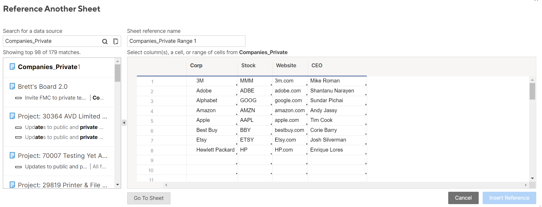
通过点击此处的列选择“Corp”列，然后将“工作表引用名称”重命名为简单的名称，如“Corp_Column”。

对每个列(“Stock_Column”，“Website_Column”)重复此步骤。确保每次完成后按“插入参考”。

---

链接“原始”工作表中的单元格

您将需要为每行的“Corp”值链接Cell值。“Corp”值是该行的Primary值。(有关Primary值的更多信息，请参见这个链接）.

要做到这一点，您可以右键单击单元格，然后选择“从其他工作表中的单元格链接”，然后找到适用的单元格。你可以选择一个单元格范围，所以在这个练习中，我们将从“company_private”表中选择Corp列范围:

(请注意，这可能会链接“原始”工作表的前50行-一旦完成此设置，您将需要删除不需要的行)

这个"Corp"值将扮演我们的"标识符，用于下面的INDEX MATCH函数。对于新的行，我们将在后面介绍。这是在处理现有的行。

--------

索引匹配函数!

我们终于到了。下面介绍如何跨多个表使用INDEX MATCH。

现在已经设置了引用，现在可以运行INDEX MATCH函数了。

以下是INDEX MATCH的工作原理:

=INDEX([要显示的数据范围]从),匹配([标识符]、[要查找标识符的范围，[排序选项])，[可选列索引])

的标识符只是可以用来将一个单元格值从一个工作表匹配到另一个工作表的东西。

对于此标识符，您应该使用始终唯一的单元格值(否则，如果有重复的值，这个公式将从它能找到的第一个值中取值)。

下面是INDEX MATCH对函数的工作原理:

使用INDEX公式的第一部分来设置数据范围你想要显示。
使用INDEX公式第二部分中的MATCH来指定什么行从中提取数据。
INDEX公式的第三部分是可选的。如果INDEX公式的第一部分包含多个列，则使用该参数指定从哪个列提取数据。对于我们的设置，你不需要担心这个。

--------

列的公式

因此，对于我们的“companyes_public”表，下面是“股票”和“网站”列的公式:

股票列公式:

=指数({Stock_Column},匹配((电子邮件保护)， {Corp_Column}， 0))

网站栏目公式

=指数({Website_Column},匹配((电子邮件保护)， {Corp_Column}， 0))

对于其中的每一个，您都需要将公式添加到顶部行，右键单击单元格，然后选择“转换为列公式”。这将公式添加到整个列中。

下面是第一个公式的工作原理:

索引“companyes_private”表中引用的“Stock_Column”范围(最终将返回我们正在寻找的值)
然后，通过搜索“companyes_private”表的“corpor_column”范围，从“companyes_public”表的“Corp”列中找到与名称匹配的行号。

“网站”一栏的公式也是如此。

基本上，它所做的是匹配行“Corp”字段中的名称，找到相邻的“Stock”值，并显示原始工作表中的“Stock”值。

要测试这一点，只需随意添加名称，看看它是否会为其他列调出正确的值，并且只要值存在，它应该永远不会给您“#NO-MATCH”错误。测试示例:

我在每一列中都添加了“(Public)”，以明确表示这来自“companyes_public”表。

--------

我可以解释如何处理新行，但那得等到下次了，因为我现在很忙。希望这篇文章能让你和其他谷歌用户在解决方案的列车上走得足够远。

布雷特埃里克 · 11/08/21

We want to clone only certain columns to make them visible to an audience. We don't want the audience to see all the columns in the original (A) Smartsheet. We tried cell linking in Smartsheet (B), but it doesn't update when new rows are added.<\/p>

Looking for a formula that will always see what's in each column of sheet A and display the data onto the other sheet (B) . I have zero experience with formulas and curious if the Index or Match would do this.<\/p>","bodyRaw":"[{\"insert\":\"We want to clone only certain columns to make them visible to an audience. We don't want the audience to see all the columns in the original (A) Smartsheet. We tried cell linking in Smartsheet (B), but it doesn't update when new rows are added.\\nLooking for a formula that will always see what's in each column of sheet A and display the data onto the other sheet (B) . I have zero experience with formulas and curious if the Index or Match would do this.\\n\"}]","format":"rich","dateInserted":"2021-10-29T17:58:40+00:00","insertUser":{"userID":141355,"name":"Donnax","url":"https:\/\/community.smartsheet.com\/profile\/Donnax","photoUrl":"https:\/\/us.v-cdn.net\/6031209\/uploads\/defaultavatar\/nWRMFRX6I99I6.jpg","dateLastActive":"2021-11-11T17:40:10+00:00","banned":0,"punished":0,"private":false,"label":"✭"},"displayOptions":{"showUserLabel":false,"showCompactUserInfo":true,"showDiscussionLink":false,"showPostLink":false,"showCategoryLink":false,"renderFullContent":false,"expandByDefault":false},"url":"https:\/\/community.smartsheet.com\/discussion\/comment\/309421#Comment_309421","embedType":"quote"}"> https://community.smartsheet.com/discussion/comment/309421#Comment_309421

嘿唐娜。

今天下午重新看了一下您的请求，我意识到Report可以满足您的要求。“受众”是否需要访问实际的工作表，或者您只是希望原始工作表中的数据子集对他们可用?因为只读报告将是完美的。

在这里阅读更多报告，并告诉我这是否可行:报告| Smartsheet学习中心

Donnax · 11/09/21

你好，他们只需要访问日历形式的查看信息。如果报表可以显示为日历，那就太棒了。

下面是我们想要看到的与原始工作表的对比。我们作为日历发布，并将其嵌入到网页中。

布雷特埃里克 · 11/11/21

@Donnax-知道了。这就是为什么你需要两张床单。日历形式的报表不可用。谢谢截图!

好的，你可以按照我上面的教程去做，这是可行的。让我们使用“课程名称”作为标识符。

我正在努力弄清楚如何输入你需要做的所有事情，所以我认为制作两张“虚拟”表格并与你分享会更容易。下面的链接。

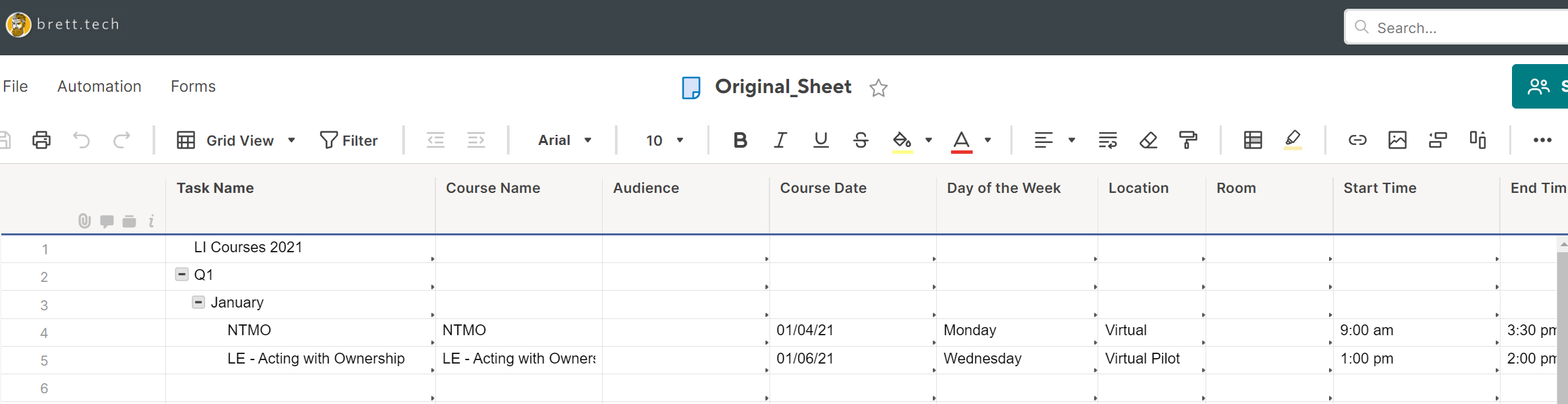
我使用了你截图中的名字:“Original_Sheet”和“Visible_to_Audience”。

Original_Sheet链接:https://app.smartsheet.com/b/publish?EQBCT=962c9006c23240e9b522f32d59e1c15d

Visible_to_Audience链接:https://app.smartsheet.com/b/publish?EQBCT=b3fe083ae08f47f58943a6c0db0ac1e0

我添加了一个“注释”列来描述我对单元格所做的工作。

----

我所做的一切都是创建多个引用来“Original_Sheet”从“Visible_to_Audience”表单我创建了一个引用到每列，我命名为“OriginalSheet_ColumnNameColumn”(即“OriginalSheet_CourseDateColumn”)。

“Visible_to_Audience”表中的表参考管理器。

然后，对于“Visible_to_Audience”表中的每个单元格，我使用INDEX/MATCH公式，就像我在上面的教程中概述的那样。

这里有一个例子:对于“Visible_to_Audience”表单上的“Course Date”列，我使用了这个公式，并将其设置为列公式：

=INDEX({OriginalSheet_CourseDateColumn}， MATCH([课程名称]@row， {OriginalSheet_TaskNameColumn}， 0))

这有道理吗?

看来你得弄清楚你想用什么来做标识符为了使这两张表正确同步。然后，您所需要做的就是创建与Identifier名称相同的新行，所有单元格都将获得正确的数据。

“Visible_to_Audience”表上的“课程名称”与“Original_Sheet”表上的“任务名称”相链接。这是我能看到的，这是我用的标识符。看起来你的“Visible_to_Audience”表上有一个过滤器，我试图模仿。它似乎也有不同的值，我看不见;因此，您需要弄清楚如何识别在INDEX/MATCH公式或某种过滤器中保留哪些“Course Name”值。

设置完成后，您需要做的就是确保您选择的“标识符”列出现在每个工作表上。对我来说，我在“Visible_to_Audience”表上使用“课程名称”，在“Original_Sheet”表上使用“任务名称”。你可能想用别的东西。

如果你需要额外的帮助，如果你愿意，我愿意免费伸出援手。给我发邮件吧(电子邮件保护)我们可以约个时间聊一聊。

‎

从另一个工作表引用多个列

答案

例子:《两张纸的故事》

Companies_Private表:

Companies_Public表:

在“新”表上创建一些对“原始”表的引用

链接“原始”工作表中的单元格

索引匹配函数!

列的公式

帮助文章参考资料欧宝体育app官方888

类别